9  Networks, Circuits, and Graphs

Synthetic biology is full of relationships.

A transcription factor activates a promoter. A repressor blocks expression of a reporter. A plasmid depends on a specific backbone. A design workflow may require one assembly step before another. A gene circuit may contain a cascade, a feedback loop, or an incoherent feed-forward motif.

Tables are still useful here, but in this chapter we will introduce another way to think about biological structure: graphs.

A graph is a collection of nodes connected by edges.

In synthetic biology, nodes might represent:

Edges represent relationships between those things.

Examples include:

Graphs help us move from “what values are in this table?” to “how is this system connected?”

In this chapter, we will learn how to represent biological relationships in Python using tidy tables and NetworkX.

9.1 Graphs as tidy data

In Chapter 5, we introduced tidy data and agreed to use it as the default tabular format from that point onward.

That convention continues here.

When we represent a network in a table, we will usually use one of two tidy tables:

  1. a node table, where each row is one node
  2. an edge table, where each row is one edge

This is a very practical habit.

A tidy edge table is easy to:

  • read from CSV
  • inspect with pandas
  • filter by interaction type
  • merge with metadata
  • save after curation
  • convert into a graph object when needed

Likewise, a tidy node table makes it easy to attach metadata like:

  • part type
  • sequence length
  • host organism
  • plasmid name
  • copy number class
  • fluorescent protein color
  • design status

So although we are introducing graph thinking, we are not abandoning tidy data.

We are adding a graph layer on top of it.

9.2 Installing NetworkX

The most widely used pure-Python graph library is networkx.

If you need to install it, the command is:

pip install networkx

We will also use pandas, which we already introduced in the previous chapter.

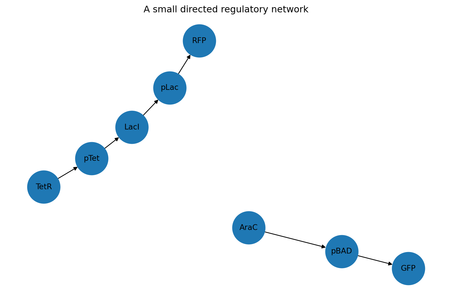
9.3 A first regulatory network

Let us begin with a simple gene regulation example.

Suppose we have a sensor circuit with these relationships:

  • AraC activates pBAD
  • pBAD drives expression of GFP
  • LacI represses pLac
  • pLac drives expression of RFP
  • TetR represses pTet
  • pTet drives expression of LacI

We can represent those relationships as a tidy edge table.

import pandas as pd

edge_table = pd.DataFrame(
    [
        {"source": "AraC", "target": "pBAD", "interaction": "activation", "sign": 1},
        {"source": "pBAD", "target": "GFP", "interaction": "expression", "sign": 1},
        {"source": "LacI", "target": "pLac", "interaction": "repression", "sign": -1},
        {"source": "pLac", "target": "RFP", "interaction": "expression", "sign": 1},
        {"source": "TetR", "target": "pTet", "interaction": "repression", "sign": -1},
        {"source": "pTet", "target": "LacI", "interaction": "expression", "sign": 1},
    ]
)

edge_table
source target interaction sign
0 AraC pBAD activation 1
1 pBAD GFP expression 1
2 LacI pLac repression -1
3 pLac RFP expression 1
4 TetR pTet repression -1
5 pTet LacI expression 1

This table is tidy because:

  • each row is one interaction
  • each column is one variable
  • the observational unit is consistent

That is the first habit to keep.

Even when we plan to use a graph library later, it is often best to store and exchange network data as tidy tables.

9.4 Building a directed graph from a tidy edge table

Many biological networks are directed.

That means an edge has a direction.

If AraC regulates pBAD, then the edge points from AraC to pBAD. The reverse is not automatically true.

We can build a directed graph with NetworkX.

import networkx as nx

G = nx.from_pandas_edgelist(
    edge_table,
    source="source",
    target="target",
    edge_attr=["interaction", "sign"],
    create_using=nx.DiGraph(),
)

G
<networkx.classes.digraph.DiGraph at 0x10db9a850>

The result is a DiGraph, which stands for directed graph.

We can inspect its basic properties.

G.number_of_nodes(), G.number_of_edges()
(8, 6)
sorted(G.nodes())
['AraC', 'GFP', 'LacI', 'RFP', 'TetR', 'pBAD', 'pLac', 'pTet']
list(G.edges(data=True))
[('AraC', 'pBAD', {'interaction': 'activation', 'sign': 1}),
 ('pBAD', 'GFP', {'interaction': 'expression', 'sign': 1}),
 ('LacI', 'pLac', {'interaction': 'repression', 'sign': -1}),
 ('pLac', 'RFP', {'interaction': 'expression', 'sign': 1}),
 ('TetR', 'pTet', {'interaction': 'repression', 'sign': -1}),
 ('pTet', 'LacI', {'interaction': 'expression', 'sign': 1})]

A graph object is useful because it lets us ask structural questions more naturally than a plain table can.

9.5 Nodes, edges, predecessors, and successors

In a directed graph:

  • a node can have incoming edges
  • a node can have outgoing edges

For a regulatory network, we often care about:

  • what does this regulator affect?
  • what controls this promoter or gene?

NetworkX gives us direct methods for that.

list(G.successors("AraC"))
['pBAD']
list(G.successors("pBAD"))
['GFP']
list(G.predecessors("pLac"))
['LacI']

This language is worth learning.

If you say that node A has B as a successor, you are saying there is a directed edge from A to B.

9.6 Using a node table for metadata

Edges tell us how nodes are connected. Node tables tell us what the nodes are.

Let us create a tidy node table.

node_table = pd.DataFrame(
    [
        {"node": "AraC", "kind": "protein", "role": "regulator"},
        {"node": "pBAD", "kind": "promoter", "role": "input promoter"},
        {"node": "GFP", "kind": "protein", "role": "reporter"},
        {"node": "LacI", "kind": "protein", "role": "repressor"},
        {"node": "pLac", "kind": "promoter", "role": "regulated promoter"},
        {"node": "RFP", "kind": "protein", "role": "reporter"},
        {"node": "TetR", "kind": "protein", "role": "repressor"},
        {"node": "pTet", "kind": "promoter", "role": "regulated promoter"},
    ]
)

node_table
node kind role
0 AraC protein regulator
1 pBAD promoter input promoter
2 GFP protein reporter
3 LacI protein repressor
4 pLac promoter regulated promoter
5 RFP protein reporter
6 TetR protein repressor
7 pTet promoter regulated promoter

We can attach this metadata to the graph.

node_attributes = node_table.set_index("node").to_dict(orient="index")
nx.set_node_attributes(G, node_attributes)

G.nodes["GFP"]
{'kind': 'protein', 'role': 'reporter'}
G.nodes["pBAD"]
{'kind': 'promoter', 'role': 'input promoter'}

This is one of the reasons tidy node tables are powerful.

They let us curate metadata in a spreadsheet-like format, then move that metadata into a graph object for analysis.

9.7 Drawing a small circuit

Graphs can be inspected numerically, but sometimes a simple diagram helps.

import matplotlib.pyplot as plt

pos = nx.spring_layout(G, seed=7)

plt.figure(figsize=(8, 5))
nx.draw(
    G,
    pos,
    with_labels=True,
    node_size=1800,
    arrows=True,
    font_size=10,
)
plt.title("A small directed regulatory network")
plt.show()

This is not a publication-quality biological diagram, but it is very useful for quick inspection.

It answers questions like:

  • are the expected nodes present?
  • is the directionality correct?
  • did we accidentally omit an interaction?
  • does the network have disconnected parts?

For quick exploratory work, simple graph drawings are often enough.

9.8 Keeping edge metadata tidy

Because we built the graph from a tidy edge table, the interaction metadata remains accessible.

for source, target, data in G.edges(data=True):
    print(f"{source} -> {target}: {data['interaction']} (sign={data['sign']})")
AraC -> pBAD: activation (sign=1)
pBAD -> GFP: expression (sign=1)
LacI -> pLac: repression (sign=-1)
pLac -> RFP: expression (sign=1)
TetR -> pTet: repression (sign=-1)
pTet -> LacI: expression (sign=1)

A good rule is this:

  • curate in tidy tables
  • analyze in graph objects
  • export results back to tidy tables when useful

That rhythm scales well.

9.9 Finding paths through a circuit

A path is a sequence of connected edges.

In synthetic biology, paths are useful when thinking about:

  • signal flow through a regulatory cascade
  • design dependencies
  • propagation of control
  • multi-step assembly or computation

Let us build a slightly richer network with a clear cascade.

cascade_edges = pd.DataFrame(
    [
        {"source": "Input", "target": "TF1", "interaction": "activation", "sign": 1},
        {"source": "TF1", "target": "TF2", "interaction": "activation", "sign": 1},
        {"source": "TF2", "target": "Reporter", "interaction": "activation", "sign": 1},
        {"source": "TF1", "target": "Reporter", "interaction": "repression", "sign": -1},
    ]
)

cascade = nx.from_pandas_edgelist(
    cascade_edges,
    source="source",
    target="target",
    edge_attr=["interaction", "sign"],
    create_using=nx.DiGraph(),
)

list(cascade.edges(data=True))
[('Input', 'TF1', {'interaction': 'activation', 'sign': 1}),
 ('TF1', 'TF2', {'interaction': 'activation', 'sign': 1}),
 ('TF1', 'Reporter', {'interaction': 'repression', 'sign': -1}),
 ('TF2', 'Reporter', {'interaction': 'activation', 'sign': 1})]

We can ask for the shortest directed path from Input to Reporter.

nx.shortest_path(cascade, source="Input", target="Reporter")
['Input', 'TF1', 'Reporter']

We can also list all simple paths.

list(nx.all_simple_paths(cascade, source="Input", target="Reporter"))
[['Input', 'TF1', 'TF2', 'Reporter'], ['Input', 'TF1', 'Reporter']]

Now we can see something interesting.

There are two routes from input to output:

  • Input -> TF1 -> Reporter
  • Input -> TF1 -> TF2 -> Reporter

That is already the structure of a small network motif.

9.10 Feed-forward logic

A feed-forward loop appears when one upstream regulator affects an output both directly and indirectly through an intermediate node.

Our example has exactly that shape.

We can inspect the signed influence of each path by multiplying the edge signs along the path.

def path_sign(graph, path):
    sign = 1
    for a, b in zip(path[:-1], path[1:]):
        sign *= graph.edges[a, b]["sign"]
    return sign

paths = list(nx.all_simple_paths(cascade, source="Input", target="Reporter"))

[(path, path_sign(cascade, path)) for path in paths]
[(['Input', 'TF1', 'TF2', 'Reporter'], 1), (['Input', 'TF1', 'Reporter'], -1)]

This is a simple but powerful idea.

Once a regulatory network is encoded as a graph with edge attributes, we can write small functions that reason about:

  • activation vs repression
  • path length
  • redundancy
  • conflicting paths
  • logic motifs

That is much harder to do robustly if the structure only exists informally in our heads.

9.11 Detecting feedback loops

Many synthetic circuits and natural regulatory systems contain feedback.

Feedback can stabilize, destabilize, amplify, or oscillate depending on the system.

Let us create a tiny feedback example.

feedback_edges = pd.DataFrame(
    [
        {"source": "LuxR", "target": "pLux", "interaction": "activation", "sign": 1},
        {"source": "pLux", "target": "LuxI", "interaction": "expression", "sign": 1},
        {"source": "LuxI", "target": "AHL", "interaction": "synthesis", "sign": 1},
        {"source": "AHL", "target": "LuxR", "interaction": "binding_activation", "sign": 1},
    ]
)

feedback = nx.from_pandas_edgelist(
    feedback_edges,
    source="source",
    target="target",
    edge_attr=["interaction", "sign"],
    create_using=nx.DiGraph(),
)

list(nx.simple_cycles(feedback))
[['pLux', 'LuxI', 'AHL', 'LuxR']]

A directed cycle is a clean structural definition of feedback.

If your graph contains a directed cycle, then some chain of influence returns to an earlier node.

That does not tell you the dynamics by itself, but it does tell you that feedback is structurally present.

9.12 When an adjacency matrix is useful

Although tidy edge tables are usually the best storage format, sometimes it is useful to convert a graph into a matrix.

An adjacency matrix records whether each node connects to each other node.

adjacency = nx.to_pandas_adjacency(cascade, dtype=int)
adjacency
Input TF1 TF2 Reporter
Input 0 1 0 0
TF1 0 0 1 1
TF2 0 0 0 1
Reporter 0 0 0 0

This representation is useful for:

  • matrix-based methods
  • exporting to certain analysis tools
  • checking connectivity patterns visually
  • teaching the connection between graphs and linear algebra

But for most data handling, a tidy edge table remains easier to work with.

That is why our default workflow remains:

  • tidy tables for storage and curation
  • graph objects for structural analysis
  • matrices only when needed

9.13 Converting a graph back into a tidy edge table

Sometimes we start with a graph, perform analysis, and then want to save the result.

We can always recover a tidy edge table.

edge_export = nx.to_pandas_edgelist(cascade)
edge_export
source target sign interaction
0 Input TF1 1 activation
1 TF1 TF2 1 activation
2 TF1 Reporter -1 repression
3 TF2 Reporter 1 activation

That means graphs do not lock us into a special format.

They are another working representation, not the final destination.

9.14 Assembly dependencies as a directed acyclic graph

Not every graph in synthetic biology is a regulatory network.

Graphs are also useful for workflows and dependencies.

Suppose a cloning workflow has these relationships:

  • the reporter cassette must be assembled before the full plasmid
  • the backbone must be prepared before the full plasmid
  • the plasmid must be sequence-verified before transformation
  • transformation must happen before induction testing

We can encode that too.

dependency_table = pd.DataFrame(
    [
        {"source": "Reporter cassette", "target": "Assembled plasmid", "dependency": "required_before"},
        {"source": "Prepared backbone", "target": "Assembled plasmid", "dependency": "required_before"},
        {"source": "Assembled plasmid", "target": "Sequence verification", "dependency": "required_before"},
        {"source": "Sequence verification", "target": "Transformation", "dependency": "required_before"},
        {"source": "Transformation", "target": "Induction test", "dependency": "required_before"},
    ]
)

dependencies = nx.from_pandas_edgelist(
    dependency_table,
    source="source",
    target="target",
    edge_attr=["dependency"],
    create_using=nx.DiGraph(),
)

list(dependencies.edges(data=True))
[('Reporter cassette', 'Assembled plasmid', {'dependency': 'required_before'}),
 ('Assembled plasmid',
  'Sequence verification',
  {'dependency': 'required_before'}),
 ('Prepared backbone', 'Assembled plasmid', {'dependency': 'required_before'}),
 ('Sequence verification',
  'Transformation',
  {'dependency': 'required_before'}),
 ('Transformation', 'Induction test', {'dependency': 'required_before'})]

This graph is intended to have no directed cycles. That kind of graph is called a directed acyclic graph, or DAG.

When a graph is a DAG, we can compute a valid execution order.

list(nx.topological_sort(dependencies))
['Reporter cassette',
 'Prepared backbone',
 'Assembled plasmid',
 'Sequence verification',
 'Transformation',
 'Induction test']

This is a beautiful example of why graph thinking matters.

The same library can help with:

  • regulatory structure
  • workflow ordering
  • assembly planning
  • analysis pipelines
  • data provenance

9.15 Detecting impossible workflows

If a dependency graph contains a cycle, the workflow is impossible as written.

For example, if step A depends on step B, step B depends on step C, and step C depends on step A, then nothing can start.

Let us create an intentionally broken workflow.

broken_dependency_table = pd.DataFrame(
    [
        {"source": "Assemble plasmid", "target": "Verify plasmid"},
        {"source": "Verify plasmid", "target": "Transform cells"},
        {"source": "Transform cells", "target": "Assemble plasmid"},
    ]
)

broken = nx.from_pandas_edgelist(
    broken_dependency_table,
    source="source",
    target="target",
    create_using=nx.DiGraph(),
)

nx.is_directed_acyclic_graph(broken)
False

Because this graph is not acyclic, a topological sort would fail.

That kind of check can prevent subtle mistakes in automation pipelines and project planning.

9.16 Merging tidy metadata with graph results

Because we began with tidy data, we can summarize graph structure and merge it back into tables.

For example, we can compute the in-degree and out-degree of each node in our first graph.

degree_summary = pd.DataFrame(
    {
        "node": list(G.nodes()),
        "in_degree": [G.in_degree(node) for node in G.nodes()],
        "out_degree": [G.out_degree(node) for node in G.nodes()],
    }
)

node_summary = node_table.merge(degree_summary, on="node", how="left")
node_summary.sort_values(["kind", "node"])
node kind role in_degree out_degree
1 pBAD promoter input promoter 1 1
4 pLac promoter regulated promoter 1 1
7 pTet promoter regulated promoter 1 1
0 AraC protein regulator 0 1
2 GFP protein reporter 1 0
3 LacI protein repressor 1 1
5 RFP protein reporter 1 0
6 TetR protein repressor 0 1

This is exactly the kind of workflow that scales well:

  1. store the network in tidy tables
  2. convert to a graph
  3. compute structural properties
  4. bring those results back into tidy tables
  5. continue analysis with pandas

That pattern will keep appearing throughout computational biology.

9.17 Choosing between a table and a graph

A good practical question is:

When should I use a table, and when should I use a graph?

Use a tidy table when you want to:

  • store curated interactions
  • edit metadata
  • merge with experimental measurements
  • save or exchange data
  • filter and summarize observations

Use a graph object when you want to:

  • follow paths
  • detect cycles
  • inspect predecessors and successors
  • compute connectivity measures
  • reason about motifs and dependencies

In practice, most good workflows use both.

9.18 Exercises

  1. Create a tidy edge table for a repressilator-like circuit with three repressors in a cycle.
  2. Convert that table into a directed graph and confirm that it contains a directed cycle.
  3. Add a tidy node table with metadata such as kind, host, or copy_number_class.
  4. Write a function that returns all direct targets of a regulator.
  5. Write a function that counts how many activating and repressing edges exist in a graph.
  6. Build a dependency graph for a DBTL workflow and compute a valid topological order.
  7. Export one of your graphs back into a tidy edge table and save it as CSV.

9.19 Recap

In this chapter, we introduced graph thinking for synthetic biology.

The most important ideas are:

  • a graph contains nodes and edges
  • many biological relationships are naturally directed
  • tidy edge tables and node tables are the best default storage format
  • networkx lets us convert tidy tables into graph objects for analysis
  • graph objects help us inspect paths, cycles, feedback, motifs, and workflow dependencies
  • after graph analysis, we can move results back into tidy tables for further work

That final point matters a lot.

We are not replacing tidy data. We are extending it.

From here onward, when we deal with network structure, pathway logic, or design dependencies, we will still prefer tidy tables as the standard exchange format, and use graph objects as computational tools on top of them.